Calibration
1. Retrieving Data from the Arduino
We used rosserial to enable the Arduino to publish the taxel data to a ROS topic, so from the ROS side, we can manage the data and visualize it in RViz. To setup the Arduino IDE to use rosserial, please see the document here.
(1) Arduino:
From the Arduino side, we read data and store it an array c[], then we publish the data to a ROS topic called "skin/taxels" with a timestamp.
ros::NodeHandle nh;
wholearm_skin_ros::TaxelData msg;
ros::Publisher pub("skin/taxels", &msg);
void loop() {
// read data and restore them in c[] array
msg.cdc = c;
msg.cdc_length = NUM_TAXELS;
msg.header.stamp = nh.now();
pub.publish(&msg);
nh.spinOnce();
}
(2) ROS:
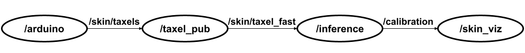
Node "/taxel_pub" gets the data which the Arduino published and then publishes it to the topic "/skin/taxel_fast" at a fixed 60HZ rate. After that, node "/inference" will tare, filter and calibrate the data (detailed methods about these three functions will be explained below) and publish it to topic "/calibration". Then, node "skin_viz" will use the cleaned data for visualization in RViz.
2. Data Preprocessing
(1) Tare
This process needs to be completed before officially starting to measure data. Additionally, throughout the taring process, the skin should not have any external forces applied to it. In this process, we will collect 100 data points from each taxel and calculate their mean values respectively. These means become the initial taxel values. Then, we subtract the calculated initial value from the measured value as the final value.
(2) Filter
sos = signal.iirfilter(2, Wn=1.5, fs=60, btype="lowpass", ftype="butter", output="sos")
We applied a second-order low-pass filter to process our data. The Butterworth filter design method was used to provide a relatively smooth response in the passband and stopband transition region. We set the cutoff frequency at 1.5 Hz, so signals below 1.5 Hz will be retained, while higher frequency signals above it will be attenuated. With a sampling rate of 60 Hz, this ensures consistency with the frequency at which we collected the capacitance data.
(3) Calibrate
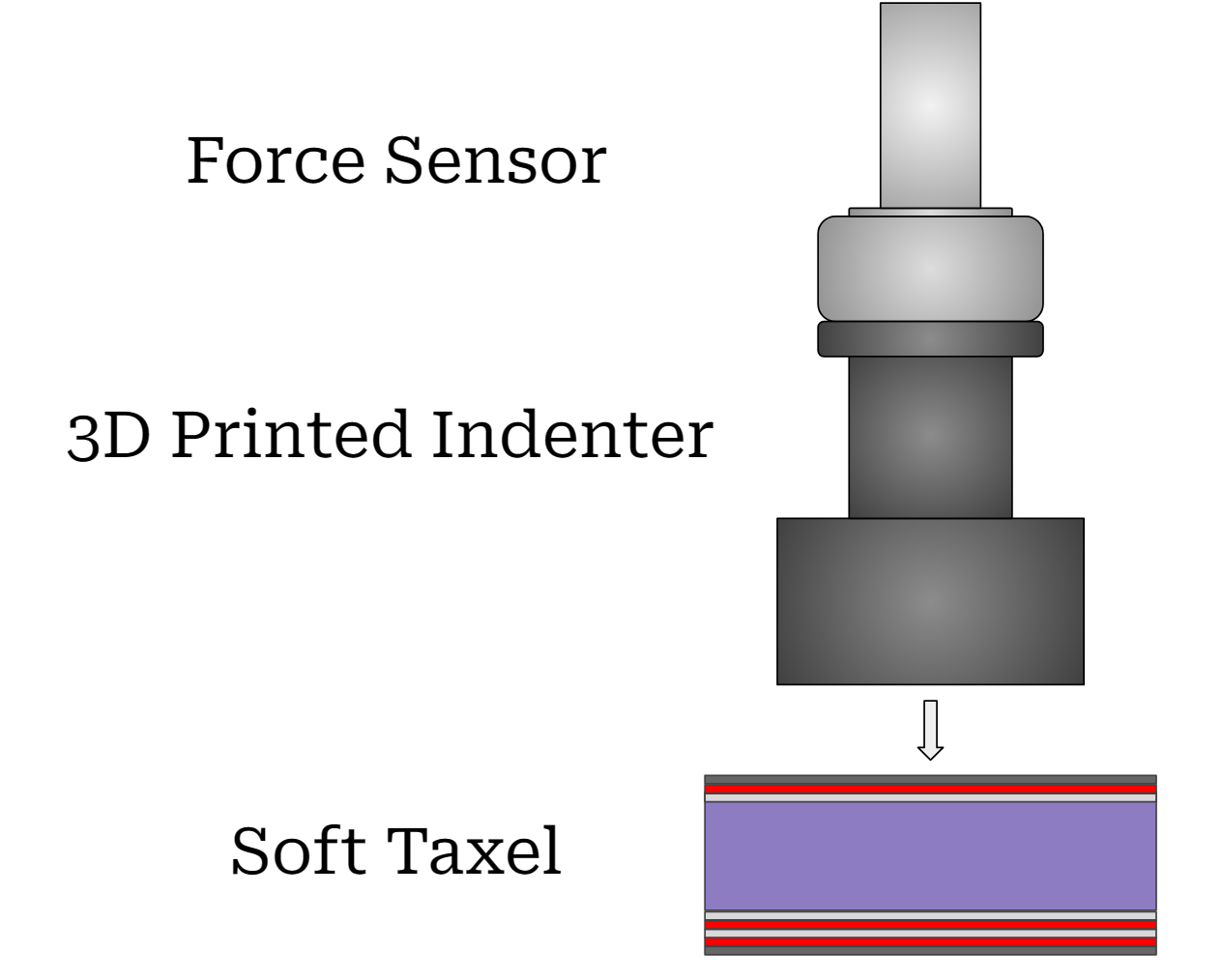
We designed a calibration function to transfer the capacitance data to force data.
In the setup shown left, we utilize an FT sensor to measure the magnitude of force. The Arduino board transmits the capacitance values detected by the taxel. We employ a robot arm to exert a fixed motion on the taxel 20 times, recording data for both force and capacitance. Subsequently, we use a third-order polynomial to fit this data, obtaining four coefficients: a4, a3, a2, and a0. With these coefficients and the measured capacitance values, we can predict the force magnitude.
msg.data[i] = self.model['a3'] + self.model['a2']*skin_data[i] + self.model['a1']*skin_data[i]**2 + self.model['a0']*skin_data[i]**3
3. Visualization
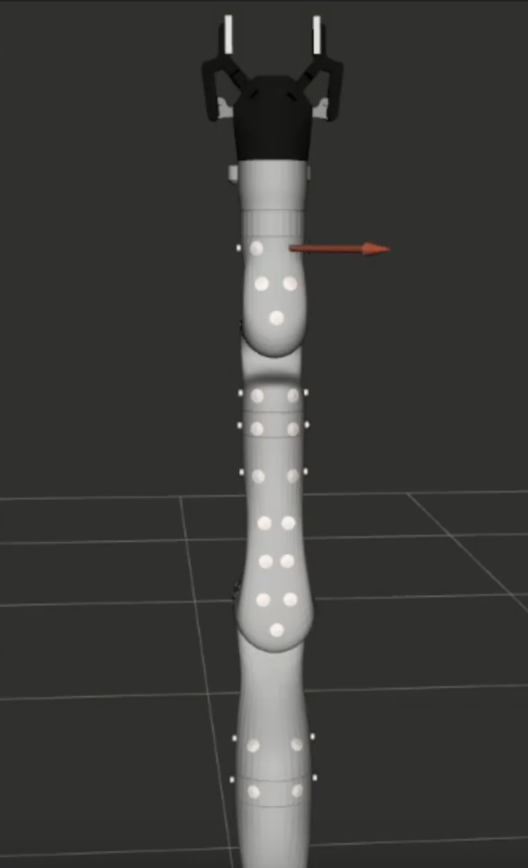
The viz_sub.py file reads in data from the calibration topic "/calibration" and publishes arrows which represent force vectors to be visualized in RViz on the "taxel_markers" topic. These arrows are normalized to fit between the range [0, 1]. The code for this visualization can be found here, and detailed documentation on how it functions can be found in this README.md.
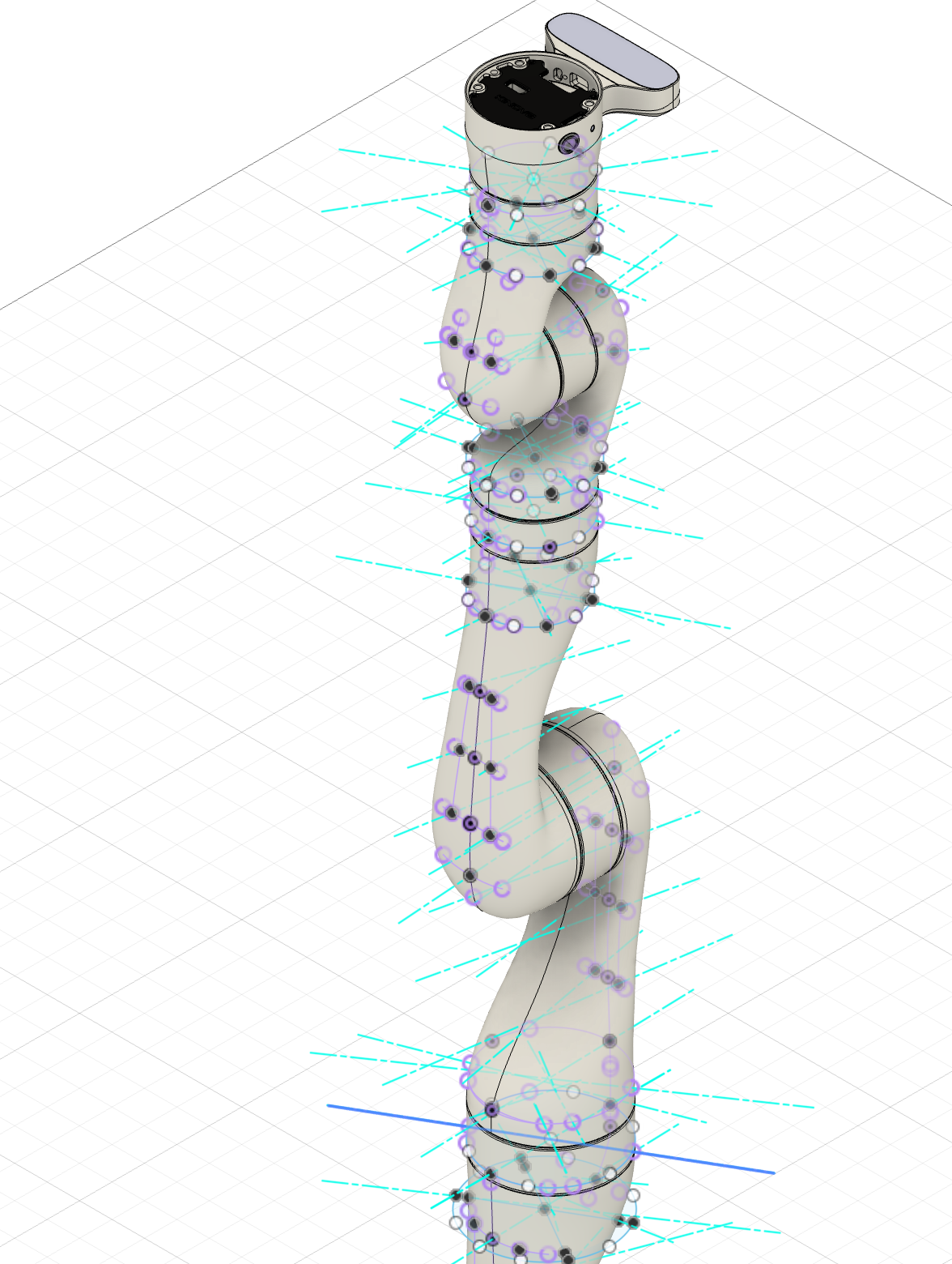
To get each taxel's position and orientation, they were modeled in Fusion 360 on our robot arm, the Kinova Gen 3 7 dof. This file is attached here for reference. The taxels are modeled as sketch points, and they do not show up in the web editor. Please click "open in Fusion 360" to see the taxels. Sketch point's with a blue axes running through them are taxels.